Analyzing rate my professor ratings

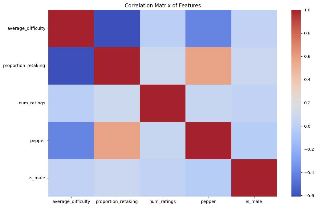
What we did: To investigate potential gender bias in professor ratings, we conducted a linear regression analysis with the dependent variable as the average rating and gender as a key predictor. We chose linear regression as we could factor in the potential confounders such as the proportion of students retaking the course, the number of online ratings, total ratings, average difficulty, and whether the professor received a "pepper" tag available in the dataset. Observations with missing values in the “proportion retaking” variable were dropped, resulting in a dataset with 919 rows (569 male and 350 female professors).

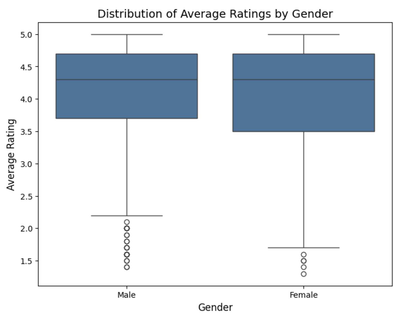
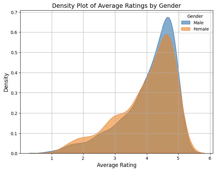
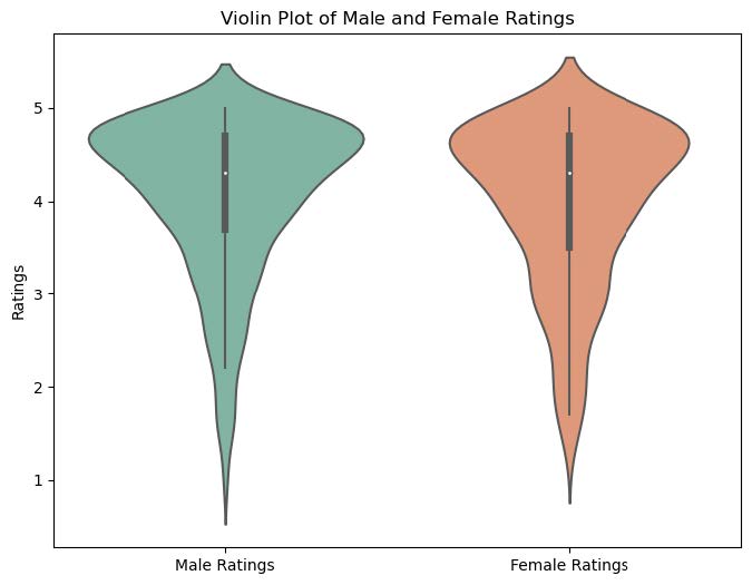
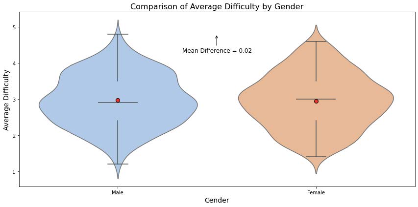
What we found: The OLS results indicate no statistically significant gender bias in average ratings. The coefficient for ‘male gender’ (-0.0057, p=0.800) suggests that, after controlling for other factors, gender does not play a meaningful role in predicting ratings (this is supported by the box plot which shows an overlapping distribution of mean ratings between male and female). On the other hand, other variables showed stronger associations with ratings. Professors with higher proportions of students retaking their courses (coef = 0.0261, p < 0.001) and those who received a ‘pepper’ tag (coef=0.2203, p < 0.001) were significantly more likely to have higher average ratings. Conversely, the average difficulty had a negative impact on ratings (coef=-0.1827, p < 0.001), reflecting that professors perceived as more difficult tended to receive lower scores.

The model captures an R-squared value of 0.853, meaning that 85.3% of the variance in ratings is explained by the included predictors. While the model captures strong associations for factors like difficulty and the "pepper" tag, gender (whether one is male) did not emerge as a significant predictor. These findings suggest that other variables discussed above have a stronger influence on professor ratings than gender. On top of what we stated above in the “Common assumptions/limitations”, this analysis assumes that the relationship between gender and average ratings is adequately captured by the included variables. Therefore, a major limitation of the conclusion is the exclusion of potential confounding variables, such as differences in academic disciplines, teaching methods, or the inherent biases of students who provide ratings etc. Additionally, the imposed threshold of 25 ratings may exclude professors with fewer reviews, potentially limiting the generalizability of the findings.

What we did: To investigate whether there is a gender difference in the variance of professor ratings, we calculated the variances of average ratings for male and female professors separately. The variance for male professors was calculated as 0.719, while for female professors, it was slightly higher at 0.787. We then used Levene's test to statistically evaluate whether these differences in variance were significant. Levene's test is suitable for comparing variances between groups as it is robust to deviations from normality.

What we found: The results of Levene's test showed a test statistic of 1.87 with a p-value of 0.172. Since the p-value is greater than the standard significance threshold of 0.005, we do not obtain evidence to drop the null hypothesis that the variances of the two groups are equal. This suggests that there is no statistically significant difference in the spread (variance) of average ratings between male and female professors, even though female professors showed slightly higher variance numerically.On top of what we stated above in the “Common Assumptions/Limitations” section, an assumption we made for the Levene’s test is that observations within the groups are independent of each other. This conclusion has limitations, including the fact that our dataset contains more male professors than female professors, which might skew the resulting variances.

What we did: To estimate the effect size of the gender bias in the average ratings as well as in the spread of the average ratings, we calculated Cohen’s D. To calculate Cohen's D between the variances, we treated the variance of males and females as the population “means”. To calculate Cohen’s D for the average rating, we used the sample means as the population means.

What we found: Cohen’s D for gender bias in the average rating was -0.11, with a 95% confidence interval of -0.023 to 0.237, which means that the difference in average ratings between male and female professors is negligible. This minimal effect size aligns with what we found in question 1 since gender is not a significant predictor of average ratings. Cohen’s D for gender bias in the spread of the average rating is -1.40 with a confidence interval of -1.54 to -1.25. This shows that the variance in male ratings is practically lower than that of the female ratings. On top of what we stated above in the “Common Assumptions/Limitations” section, a limitation for this analysis is that in reality, we would have used different measures to calculate the effect size for variances and linear regression, but for this project, Cohen's D was condoned.

What we did: To determine if there is a gender difference in the tags awarded by students, we merged the numerical dataset with the tags dataset and conducted a Mann-Whitney U test on each of the tag columns to test possible differences in central tendency. With an alpha level of 0.005, our null hypothesis was no difference between males and females in the median number of normalized tags per category, whereas our alternative hypothesis was that there exists a significant difference.

What we found: The 3 most gendered (lowest p-value) tags are ‘Hilarious’ (U Statistic = 140543.5, p-value = 7.343214e-13), ‘Respected’ (U Statistic = 129805.5, p-value = 4.271263e-06), and ‘Extra Credit’ (U Statistic = 93699, p-value = 5.935096e-05). Each of the most gendered tags exhibits p-values below our alpha level of 0.005. The plot on the left shows the distribution of ratings for the “Hilarious” tag split by 3 male and female. Furthermore, the 3 least gendered tags are ‘Pop Quizzes!’ (U Statistic = 108246.5, p-value = 0.535528), ‘Lecture Heavy’ (U Statistic = 112616.5, p-value = 0.595073), and ‘Tough grader’ (U Statistic = 110058, p-value = 0.935189). Each of the least gendered tags exhibits p-values above our alpha level of 0.005. For p-values below our alpha threshold, we conclude a statistically significant difference in the median of the normalized tag by gender. For p-values above our threshold, there is insufficient evidence to conclude that there exists a statistically significant difference. On top of what we stated above in the “Common Assumptions/Limitations” section, we may violate an assumption of the Mann-Whitney U test if the shapes of the distributions are not highly similar for each tag. Additionally, the ratings of the two groups might not be independent (e.g., there may be gendered social circles in a class, and students’ opinions of the professor may be influenced by their social circles). Another limitation is the multiple testing problem as we are performing many tests simultaneously on the same dataset.

What we did: To determine if there is a gender difference in average difficulty, we conducted a Mann-Whitney U test to test a possible difference in central tendency. With an alpha level of 0.005, our null hypothesis was that there was no difference between males and females in the median score of average difficulty, whereas our alternative hypothesis was that there exists a significant difference.

What we found: We found a U Statistic of 112107.5 and a p-value of 0.6858. Given a p-value above our alpha threshold, there is insufficient evidence to conclude that there exists a gender difference in the median score of average difficulty. On top of what we stated above in the “Common Assumptions/Limitations” section, we may violate an assumption if the shapes of the distributions are not highly similar for each tag. Additionally, the ratings of the two groups might not be independent (e.g., there may be gendered social circles in a class, and students’ opinions of the professor may be influenced by their social circles). On top of what we stated above in the common assumptions/limitations, one potential limitation is that our 25-rating threshold might select professors who tend to be perceived as more difficult - for instance, students might be more inclined to rate more polarizing professors.

What we did: To quantify the likely size of this effect at 95% confidence, we calculated Cohen’s d. To calculate Cohen’s d for the average difficulty, we used the sample means in place of the population means.

What we found: Cohen’s d for gender difference in the average difficulty was 0.0289, with a 95% confidence interval of -0.1009 to 0.1587, which means that the difference in average difficulty between male and female professors is practically negligible. This makes sense, as the Mann-Whitney U test did not exhibit a statistically significant result in the previous question. A limitation is 4 that in reality we would have used different measures to calculate effect size for non-cardinal data, but Cohen's d was condoned for this project. On top of what we stated above in the common assumptions/limitations, one potential limitation, similar to the previous question, is that our 25-rating threshold might select professors who tend to be perceived as more difficult - for instance, students might be more inclined to rate more polarizing professors.

What we did: We built multiple regression models (linear, Lasso, and Ridge) to predict professors' average ratings based on numerical predictors, including average difficulty, proportion retaking, number of ratings, pepper, male gender, and number of ratings from online classes. Before fitting the models, we performed data preprocessing, including dropping NAs in the proportion retaking column(leading to 919 data points - 569 males and 350 females) and addressing potential collinearity. Variance Inflation Factors (VIFs) were re-computed to confirm collinearity was mitigated, as VIF values of all remaining features were below 2.5. The correlation matrix (as shown in the heatmap) also supports this, with the highest correlation coefficient between “pepper” and “proportion retaking” approximately at 0.4.

What we found: The regression models demonstrated strong predictive performance, with all three achieving an R² of approximately 0.87 and an RMSE around 0.31 on the test data. Across all models, ‘proportion retaking’ emerged as the most impactful predictor, with a positive coefficient around 0.61, suggesting that courses with more students retaking them tend to receive higher ratings. This makes sense as we could expect popular classes to have better ratings. In contrast, ‘average difficulty’ consistently showed a significant negative relationship with ratings, with coefficients between -0.12 and -0.13, indicating that more challenging courses are associated with lower evaluations. The pepper variable also positively influenced ratings, though to a smaller degree, while other predictors, such as ‘number of ratings’ and ‘male gender’, had minimal effects. Regularized models, such as Ridge and Lasso, produced similar results to the Linear Regression model, confirming the robustness of the feature selected and the limited degree of multicollinearity. On top of what we stated above in the “Common Assumptions/Limitations” section, this analysis assumes that the predictors included in the models adequately capture the primary drivers of average ratings and that the relationships 5 between variables are linear. A limitation of the analysis is the exclusion of qualitative or contextual factors that may also influence ratings.

What we did: We analyzed the relationship between qualitative tags and professors' average ratings using Ridge Regression, Lasso Regression, and OLS Regression. To account for multicollinearity, tags with high Variance Inflation Factors (VIF) - ‘caring’ and ‘respected’ - were excluded from the analysis. Their high correlation is also visible in the heatmap below. On top of the filters we imposed as described in the preprocessing section, we further dropped rows that contain NAs, resulting in a 919-row dataset with 569 males and 350 females. The remaining tags were used as predictors to train and evaluate the models. We conducted hyperparameter tuning for Ridge and Lasso models to determine the best parameters.

What we found: As the above table shows, all three models performed similarly, explaining roughly 80% of the variances in average ratings. The most predictive tags, consistent across all models, included ‘tough grader’ (negative coefficient at around -0.25, OLS’s p-value at 6.472609e-23), ‘amazing lectures’ (positive coefficient at approximately 0.186, OLS’s p-value at 5.819230e-17), and ‘good feedback’ (positive coefficient at around 0.175, OLS’s p-value at 5.974924e-09). The coefficients suggest that students likely favor professors who provide engaging lectures and constructive feedback while penalizing those perceived as tough graders. Other significant predictors included ‘lecture heavy’ and ‘lots of homework’, both negatively associated with ratings, indicating that workload also influences students' perceptions. On top of what we stated above in the “Common Assumptions/Limitations” section, an assumption we made here is that there are the tags included in the regressions are not dependent, but they are likely correlated in practice (e.g. ‘Good feedback’ and ‘inspirational’ might be highly correlated), this also imposes a limitation on our conclusion since the analysis might be biased by unaccounted intersections between variables.

What we did: We ran Ridge, Lasso and OLS regression on the tags data to predict average difficulty. We again removed the ‘caring’ and ‘respected’ tags due to their high correlation with other tags in order to address collinearity issues. Apart from their high correlation they also had the highest VIF, as shown below. We dropped any na’s in the resulting dataframe of tags (without ‘caring’ and ‘respected’) and average difficulty. For ridge and lasso regression, we tried alpha parameters of 0.1, 1.0, 10.0, 100.0 and 200.0.

What we found: We found that it was much harder to predict average difficulty from the tags alone, as the R2 for the OLS, Ridge and LASSO models were 0.65, 0.65 and 0.54 respectively as shown in the table below, so we could only account for 65% of the variance of the difficulty as opposed to 80% of the variance of the ratings above. The tags that most strongly predicted average difficulty from the OLS model were ‘tough grader’ (coefficient = 0.310), ‘accessible’ (coefficient = 0.137) and ‘test heavy’ (coefficient = 0.119). On top of what we stated above in the “Common Assumptions/Limitations” section, an assumption we made here is that there are the tags included in the regressions are not dependent, but they are likely correlated in practice (e.g. ‘Good feedback’ and ‘inspirational’ might be highly correlated), this also imposes a limitation on our conclusion since the analysis might be biased by unaccounted intersections between variables.

What we did: We ran a logistic regression model to predict the odds that a professor would receive a pepper or not. We dropped the “Female” column as it would produce collinearity problems if combined as a feature with the “Male” column. Both numerical and the tags were scaled according to the normalisation described at the start.

What we found: The logistic model produced an AUROC of 0.9085, indicating a good model. (The AUROC curve is shown below). The features that had the highest coefficients were “Inspirational” (1.944), “Amazing lectures” (1.5378), and “Average Rating” (1.442), and the features with the lowest coefficients were “Lecture heavy”(-0.4476), “Lots of homework” (-0.5069), and “Accessible” (-0.8455). 7 Although this correlation does not imply any causation (i.e., having amazing lectures does not mean the professor will receive a pepper), it is interesting to note that a higher pepper score is more correlated with positive attributes (inspirational, amazing lectures, etc) whilst not receiving a pepper is correlated with less positive tags such as lots of homework, lecture heavy, and being “accessible”.